uni/year2/semester1/logseq-stuff/pages/Discrete Probability Distributions%3A Binomial & Poisson.md

• #ST2001 - Statistics in Data Science I
• Previous Topic: Random Variables
• Next Topic: The Normal Distribution
• Relevant Slides:
• Often, the observations generated by different statistical experiments have the same type of behaviour.
  • In general, only a handful of important probability distributions are needed to describe many of the discrete random variables encountered in practice.

• Bernoulli Trials

  collapsed:: true
  • What is a Bernoulli Trial? #card card-last-interval:: -1 card-repeats:: 1 card-ease-factor:: 2.5 card-next-schedule:: 2022-11-15T00:00:00.000Z card-last-reviewed:: 2022-11-14T20:08:48.931Z card-last-score:: 1
    • A Bernoulli Trial is a random experiment with just two outcomes - success / failure.
    • For a single trial, random variable:
      • X = \begin{cases}1, & \text{success,} \\0, & \text{failure.}\end{cases}
      • P(X = 1) = p and P(X=0) = 1 -p, where p is the success probability, or more compactly:
        • P(X = x) = p^x{(1-p)^{1-x}} \ \ \ \ \ x = 0,1
  • What is the expected value of a Bernoulli Trial? #card card-last-interval:: -1 card-repeats:: 1 card-ease-factor:: 2.5 card-next-schedule:: 2022-11-15T00:00:00.000Z card-last-reviewed:: 2022-11-14T16:20:53.147Z card-last-score:: 1
    • E[X] = (0)(1-p)+(1)p = p
  • What is the variance of a Bernoulli Trial? #card card-last-interval:: -1 card-repeats:: 1 card-ease-factor:: 2.5 card-next-schedule:: 2022-11-15T00:00:00.000Z card-last-reviewed:: 2022-11-14T16:24:49.061Z card-last-score:: 1
    • Var(X) = p(1-p)

  • Bernoulli Trial Assumptions #card

    card-last-interval:: -1 card-repeats:: 1 card-ease-factor:: 2.5 card-next-schedule:: 2022-11-15T00:00:00.000Z card-last-reviewed:: 2022-11-14T16:24:43.818Z card-last-score:: 1
    • The outcomes of the trials are mutually independent.
    • The probability of success p is constant over trials.
    • Note that these assumptions may not always be appropriate assumptions.

  • Example: Camera Flash Tests

    id:: 6368f276-bc7e-4d91-b7fb-c5b34c4c6feb
    • The time to recharge the flash is tested in three mobile phone cameras. The probability that a camera passes the test is 0.8, and the cameras perform independently. background-color:: green
    • The random variable X denotes the number of cameras that pass the test. The last column of the tables shows the values of X assigned to each outcome of the experiment. background-color:: green
    • What is the probability that the first & second cameras pass the test, and the third one fails? background-color:: green
      • 
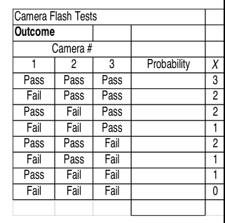
      • Each camera test can be treated as a Bernoulli Trial.
        • P(PPF) = (0.8)(0.8)(0.2) = 0.128
    • What is the probability that two cameras pass the test in three trials? background-color:: green
      • How many ways can this event happen?
        • \binom{n}{r} = \frac{n!}{r!(n-r)!} = \frac{3!}{2!(3-2)!} = 3
      • What is the probability of this event?
        • 0.128 for each of the three ways.
        • Probability = 3(0.128) = 0.383.
      • This is an example of the Binomial Distribution.

• The Binomial Distribution

  • What is a binomial random variable? #card card-last-interval:: -1 card-repeats:: 1 card-ease-factor:: 2.5 card-next-schedule:: 2022-11-15T00:00:00.000Z card-last-reviewed:: 2022-11-14T20:25:45.051Z card-last-score:: 1
    • A random experiment consists of n Bernoulli trials such that:
      • 1. The trials are independent.
        2. Each trial results in only two possible outcomes, labelled as "success" & "failure".
        3. The probability of a success in each trial, denotes as p, remains constant.
    • The random variable X that equals the number of trials that result in a success has a binomial random variable with parameters 0 < p < 1 and n = 1, 2, \cdots.
    • The probability mass function of X is
      • f(x) = \binom{n}{x}p^x (1-p)^{n-x} \ \ \ \ \ x = 0,1,\cdots, n

  • Example: Camera Flash Tests

    • See ((6368f276-bc7e-4d91-b7fb-c5b34c4c6feb)) for whole question. background-color:: green
    • Calculate the probability of 2 passes in 3 tests. background-color:: green
      • We are given that n = 3 and p = 0.8.
      • Use the Binomial Distribution formula where X is the number of passes:
        • P(X = 2) = \binom{3}{2}(0.8)^2(0.2)^1 = 3(0.128) = 0.384

  • Example: Organic Pollution

    id:: 6368f570-83e7-4642-a881-7ccd40bb0399
    • Each sample of water has a 10% chance of containing a particular organic pollutant. Assume that the sample are independent with regard to the presence of the pollutant. background-color:: green
    • Find the probability that, in the next 18 samples, exactly 2 contain the pollutant. background-color:: green
      • Let X denote the number of samples that contain the pollutant in the next 18 samples analysed. Then X is a binomial random variable with p = 0.1 and n = 18.
      • P(X = 2) = \binom{18}{2}(0.1)^2(0.9)^{18-2} = 153(0.1)^2(0.9)^16 = 0.2835
    • Determine the probability that 3 \leq X < 7. background-color:: green
      • X = 3,4,5,6
      • P(3 \leq X < 7) = P(X=3) + P(X=4) + P(X=5) + P(X=6)
      • \text{or}
      • P(3 \leq X < 7) = \sum^6_{x=3} \binom{18}{x}(0.1)^x(0.9)^{18-x}
      • = 0.168 + 0.070 + 0.022 + 0.005 = 0.265

  • Binomial Distributions in R

    card-last-interval:: -1 card-repeats:: 1 card-ease-factor:: 2.5 card-next-schedule:: 2022-11-15T00:00:00.000Z card-last-reviewed:: 2022-11-14T16:21:52.419Z card-last-score:: 1
    • dbinom(x, size, prob), where x is the number of events required, size is the total number of trials, & prob is the probability of the event occurring.

    • Example: Organic Pollution

      • In ((6368f570-83e7-4642-a881-7ccd40bb0399)), x=2, size=18, & p=0.10. background-color:: green

        • dbinom(x=2, size=18, prob=0.1)
          [1] 0.2835121
          

  • Binomial Mean & Variance #card

    card-last-interval:: -1 card-repeats:: 1 card-ease-factor:: 2.5 card-next-schedule:: 2022-11-22T00:00:00.000Z card-last-reviewed:: 2022-11-21T13:08:26.634Z card-last-score:: 1
    • If X is a binomial random variable with parameters p & n:
      • The mean & variance of the binomial distribution b(x; n,p) are
        • \mu = np \text{ and } \sigma^2 = npq \text{, where } q = 1-p

  • Chebyshev's Inequality

    • What is Chebyshev's Inequality? #card card-last-interval:: -1 card-repeats:: 1 card-ease-factor:: 2.5 card-next-schedule:: 2022-11-15T00:00:00.000Z card-last-reviewed:: 2022-11-14T16:23:31.513Z card-last-score:: 1
      • Chebyshev's Inequality provides an estimate as to where a certain percentage of observations will lie relative to the mean once the standard deviation is known.
      • For example, at least 75% of values will lie within two standard deviations of the mean.

• Poisson Distribution

  • What are Poisson Experiments? #card card-last-interval:: -1 card-repeats:: 1 card-ease-factor:: 2.5 card-next-schedule:: 2022-11-22T00:00:00.000Z card-last-reviewed:: 2022-11-21T13:05:40.034Z card-last-score:: 1
    • Experiments yielding numerical values of a random variable X, the number of outcomes occurring during a given time interval or in a specified region, are called Poisson Experiments.
    • The given time interval may be of any length, such as a minute, a day, a week, a month, or even a year.
    • A Poisson Experiment is derived from the Poisson Process and possesses the following properties:
      • The number of outcomes occurring one time interval or specified region of space is independent of the number that occur in any other disjoint time interval or region. In this sense, we say that the Poisson Process "has no memory".
      • The probability that a single outcome will occur during a very short time interval or in a small region is proportional to the length of the time interval or the size of the region, and does not depend on the number of outcomes occurring outside this time interval or region.
      • The probability that more than one outcome will occur in such a short time interval or fall in such a small region is negligible.
  • What is the Poisson Distribution? #card card-last-interval:: -1 card-repeats:: 1 card-ease-factor:: 2.5 card-next-schedule:: 2022-11-22T00:00:00.000Z card-last-reviewed:: 2022-11-21T13:06:55.129Z card-last-score:: 1
    • The random variable X that equals the number of events in a Poisson Process is a Poisson Random Variable with parameter \lambda > 0, and the probability density function is
      • f(x) = \frac{e^{-\lambda}\lambda^x}{x!} \text{ for } x = 0,1,2,3,\cdots

  • Mean & Variance of Poisson Distribution

    • If \lambda is the average number of successes occurring in a given time interval or region in the Poisson Distribution, then the mean & the variance of the Poisson distribution are both equal to \lambda.
      • Mean = \lambda, variance = \lambda.
    • A one parameter distribution.

  • Poisson Density Functions for Different Means

    • 
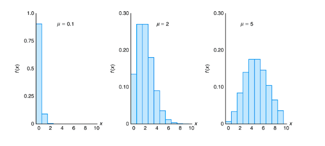
    • If the variance is much greater than the mean, then the Poisson Distribution would not be a good model for the distribution of the random variable.

  • Poisson Example: Calculations for Wire Flaws

    • Suppose that the number of flaws on a thin copper wire follows a Poisson Distribution with a mean of 2.3 flaws per millimetre. background-color:: green
    • Find the probability of exactly 2 flaws in 1mm of wire. background-color:: green
      • P(X = 2) = \frac{e^{-2.3}2.3{2}}{2!} = 0.265

  • Poisson Example: Car Park

    • A car park has 3 entrances, A, B, & C. The number of cars per hour entering through each of these is Poisson-distributed with mean \lambda_A = 1.5, \lambda_B = 1.0, and \lambda_C = 2.5. Arrivals at each entrance are independent. background-color:: green
      • T is the total number of cars entering in an hour.
      • T \sim \text{ Poisson}(\lambda_A + \lambda_B + \lambda_C) \equiv \text{Poisson}(1.5 + 1.0 + 2.5) \equiv \text{Poisson}(5)
      • P(T = 4) = \frac{e^{-5} 5^4}{4!} = 0.1755

  • Sum of Independent Poisson Random Variables #card

    card-last-interval:: -1 card-repeats:: 1 card-ease-factor:: 2.5 card-next-schedule:: 2022-11-15T00:00:00.000Z card-last-reviewed:: 2022-11-14T15:54:18.796Z card-last-score:: 1
    • If X_1, X_2, \cdots, X_n are independently Poisson distributed with parameters \lambda_1, \lambda_2, \cdots, \lambda_n then
      • T = X_1 + X_2 + \cdots + X_n \text{ is Poisson}(\lambda_1 + \lambda_2 + \cdots + \lambda_n)
    • and
      • E[T] = \lambda_1 + \lambda_2 + \cdots + \lambda_n
    • and
      • \text{Var}(T) = \lambda_1 + \lambda_2 + \cdots + \lambda_n