uni/year2/semester1/logseq-stuff/pages/Correlation & Linear Regression.md

• #ST2001 - Statistics in Data Science I
• Previous Topic: Hypothesis Testing
• Next Topic: No next topic.
• Relevant Slides:

• Modelling Relationships

  • In may applications, we want to know if there is a relationship between variables.
  • What is Regression? #card card-last-interval:: -1 card-repeats:: 1 card-ease-factor:: 2.5 card-next-schedule:: 2022-11-18T00:00:00.000Z card-last-reviewed:: 2022-11-17T19:35:13.517Z card-last-score:: 1
    • Regression is a set of statistical methods for estimating the relationship between a response variable & one or more explanatory variables.
    • Regression may have the aim of explanation (describing & quantifying relationships between variables) or prediction (how well can we predict a response variable from explanatory variables).

• Correlation Coefficients

  • What is the Sample Correlation Coefficient? #card card-last-interval:: -1 card-repeats:: 1 card-ease-factor:: 2.5 card-next-schedule:: 2022-11-18T00:00:00.000Z card-last-reviewed:: 2022-11-17T19:35:19.270Z card-last-score:: 1
    • The Sample Correlation Coefficient r gives a numerical measurement of the strength of the linear relationship between the explanatory & response variables.
    • r = \frac{\sum (x_i = \bar x)(y_i - \bar y)}{\sqrt{\sum (x_i - \bar x)^2 \sum (y_i - \bar y)^2}}
  • Note: \rho is the population correlation coefficient, while r is the sample correlation coefficient.
  • \rho = +1 means a perfect, linear direct relationship between X & Y.
  • \rho = 0 means no linear relationship between X & Y.
  • \rho = -1 means a perfect, inverse linear relationship between X & Y.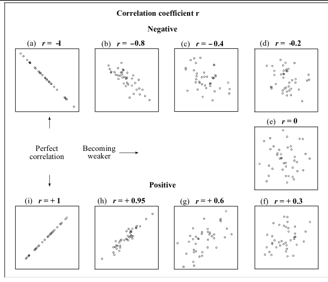
    • 
    • {:height 305, :width 645}
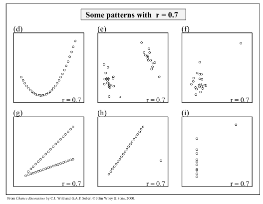    • {:height 524, :width 645}
  • Correlation treats x & y symmetrically - the correlation of x with y is the same as the correlation of y with x.
  • Correlation has no units.
  • Correlation is not affected by changes in the centre or scale of either variable.
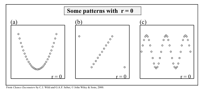
  • The correlation coefficient only measures linear association.
  • The correlation coefficient can be misleading when outliers are present.

  • Correlation \neq Causation

    • Correlation does not imply causation.
      • Scatterplots & correlation coefficients never prove causation.
    • A hidden variable that stands behind a relationship & determines it by simultaneously affecting the other two variables is called a lurking or confounding variable.
    • Don't say "correlation" when you mean "association".
      • More often than not, people say "correlation" when they mean "association".
      • The word "correlation" should be reserved for measuring the strength & direction of the linear relationships between two quantitative variables.

  • Summary

    • Scatterplots are useful graphical tools for asserting direction, form, strength, & unusual features between two variables.
    • Although not every relationship is linear, when the scatterplot is straight enough, the correlation coefficient is a useful numerical summary.
      • The sign of the correlation tells us the direction of the association.
      • The magnitude of the correlation tells us the strength of a linear association.
      • Correlation has no units, so shifting or scaling the data, standardising, or swapping the variables has no effect on the numerical value.

• Simple Linear Regression

  • What is Simple Linear Regression? #card card-last-interval:: -1 card-repeats:: 1 card-ease-factor:: 2.5 card-next-schedule:: 2022-11-18T00:00:00.000Z card-last-reviewed:: 2022-11-17T19:34:38.355Z card-last-score:: 1
    • Simple Linear Regression is the name given to the statistical technique that is used to model the dependency of a response variable on a single explanatory variable.
      • The word "simple" refers to the fact that a single explanatory variable is available.
    • Simple Linear Regression is appropriate if the average value of the response variable is a linear function of the explanatory, i..e, the underlying dependency of the response on the explanatory appears linear.

  • Strategy

    • 1. Propose a model
      2. Check the assumptions.
      3. Make some predictions.
      • The predicted value is often referred to as \hat y.
    • 4. Assess how useful it is.
      5. Improve it.

  • Interpreting the Slope & Intercept #card

    card-last-interval:: -1 card-repeats:: 1 card-ease-factor:: 2.5 card-next-schedule:: 2022-11-18T00:00:00.000Z card-last-reviewed:: 2022-11-17T19:34:57.106Z card-last-score:: 1
    • b_1 is the slope, which tells us how rapidly \hat y changes with respect to x.
      • e.g., what is the change in the mean current per unit increase in wind speed.
    • b_0 is the y-intercept, which tells us where the line intercepts the $y$-axis when x is 0.
      • e.g., what is the mean current when the wind speed is 0.

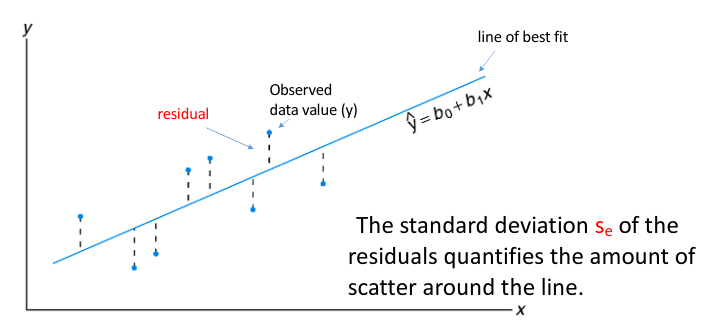
    • The Residual Standard Deviation (s_e) #card

      card-last-interval:: -1 card-repeats:: 1 card-ease-factor:: 2.5 card-next-schedule:: 2022-11-18T00:00:00.000Z card-last-reviewed:: 2022-11-17T19:35:04.870Z card-last-score:: 1
      • The standard deviation of the residuals s_e (also known as the residual standard error) measures how much the points spread around the regression line.
      • You can interpret s_e in the context of the data set -it is the typical error in the predictions made by the regression line.
    • The line of best fit is the line for which the sum of the squared residuals is the smallest, the least squares line.
      • Some residuals are positive, others are negative, and on average, they cancel each other out.
      • You can't assess how well the line fits by adding up all the residuals.
      • ()

  • Simple Linear Regression Model

    • Y_i = \beta_0 + \beta_1 x_i + \epsilon_i \text{ for } i =1, \cdots, n \text{ assuming } \epsilon_i \sim N(0, \sigma_e)

    • Features of this Model

      • $\beta_o£ (intercept) and \beta_1 (slope) are the population parameters of the model & must be estimated from the data as b_0 (sample intercept) and b_1 (sample slope).